

High-quality geometric camera calibration with active targets

Alexey Pak, High Stake GmbH (alexey.pak@high-stake.de)
Haid-und-Neue-Straße 7, 76131 Karlsruhe, Germany
Abstract
In this study, we compare the state-of-the-art camera calibration methods to those enabled by the method of active targets (MAT). Using a high-quality experimental setup, we calibrate an industrial camera to sub-mm accuracy and evaluate the resulting quality. Compared to the baseline OpenCV calibration based on static targets, MAT universally improves all quality metrics even when the same OpenCV model is calibrated. The ultimate quality is achieved by a custom free-form model, with the residual errors on the target reaching consistently the level of 10 µm. In custom tests of extrinsic parameters, MAT-based methods again prove superior and agree to respective expectations at a similar level.
1 Introduction
The method of active targets (MAT) is known to deliver superior data for geometric camera calibration [12, 5, 7]. In particular, rich and dense MAT data enable free-form camera models (FFMs), which supposedly fit the imaging geometries of cameras better than small parametric models that support only a few distortion coefficients [9, 8, 4, 13, 6]. These claims of improved quality, however, have so far been mainly supported by anecdotal or non-conclusive evidence with crude metrics [12]. In some (relatively simple) experiments they have even been shown to provide no tangible benefits at all [11]. Here we present a few experiments, intended to adequately test the limits of MAT and FFMs in comparison to the established state of the art, and derive quantitative statements about their performance in fair “apples-to-apples” comparisons.
2 Hardware setup and design of experiments
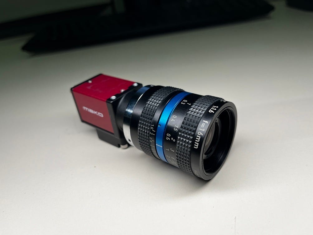
As the central object of our study, we have chosen a high-quality industrial camera, MAKO G-507 B from Allied Vision Technologies. It has a monochromatic CMOS sensor with the diagonal of 11.1 mm, the resolution of 2464 x 2056 pixels (i.e., the pixel pitch is 3.45 µm x 3.45 µm), and records data with 12-bit image bit depth. The camera is coupled with a 16 mm LINOS MeVis-C lens (Fig. 1(a)). Such combination is quite typical for industrial computer vision applications. Its field of view roughly matches our target size from the distance of 0.5 - 0.7 m, which allows us to conveniently fit the entire experimental setup on a desk.
The calibration target is a 32-inch flat LCD screen (AOC U3277PWQU) with a 4K IPS matrix (3840 x 2160 pixels). In its documentation, the sizes of the active area are specified to within 10 µm as 698.40 mm x 392.85 mm, which is sufficiently accurate for our purposes. The screen displays grayscale coded patterns, and the camera captures respective frames.
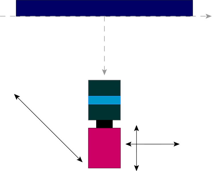
As shown in Fig. 1(b), our global system of coordinates is aligned with the screen, its origin is fixed at the geometric center of the active area (on the front glass surface). The camera directly faces the screen and may be positioned arbitrarily or attached to either of the two precision mechanical stages. These may move along the axes 1, 2, or 3 linearly without rotation.
Apart from these main components, some auxiliary parts are shown in Fig. 2(a). In particular, the screen and the camera mounts are attached to the common aluminium frame in order to reduce the sensitivity to vibrations. The 2-axis micrometric platform, aligned approximately along the global x- and z-axes (axes 1 and 2), has the full movement ranges of 26 mm and 51 mm, respectively. A single tick on each control knob corresponds to a 10 µm displacement.
The axis 3 is implemented with an optical “dovetail” rail, attached to the frame at some arbitrary angle to the screen. The position of the slider here can be determined only to 1 - 2 mm,
but we consider the rail itself sufficiently accurate for the respective camera positions to lie on (or close to) a straight line in 3D. The full range of slider movement is 250 mm. At the “arbitrary” positions inside the machine, mentioned above, the camera is fixed on an adjustable photographic arm (not shown in the photos). When in use, it is also attached to the frame.
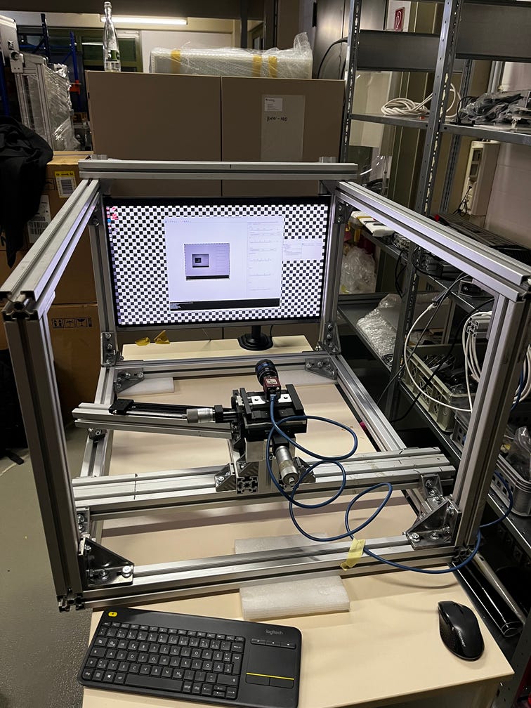
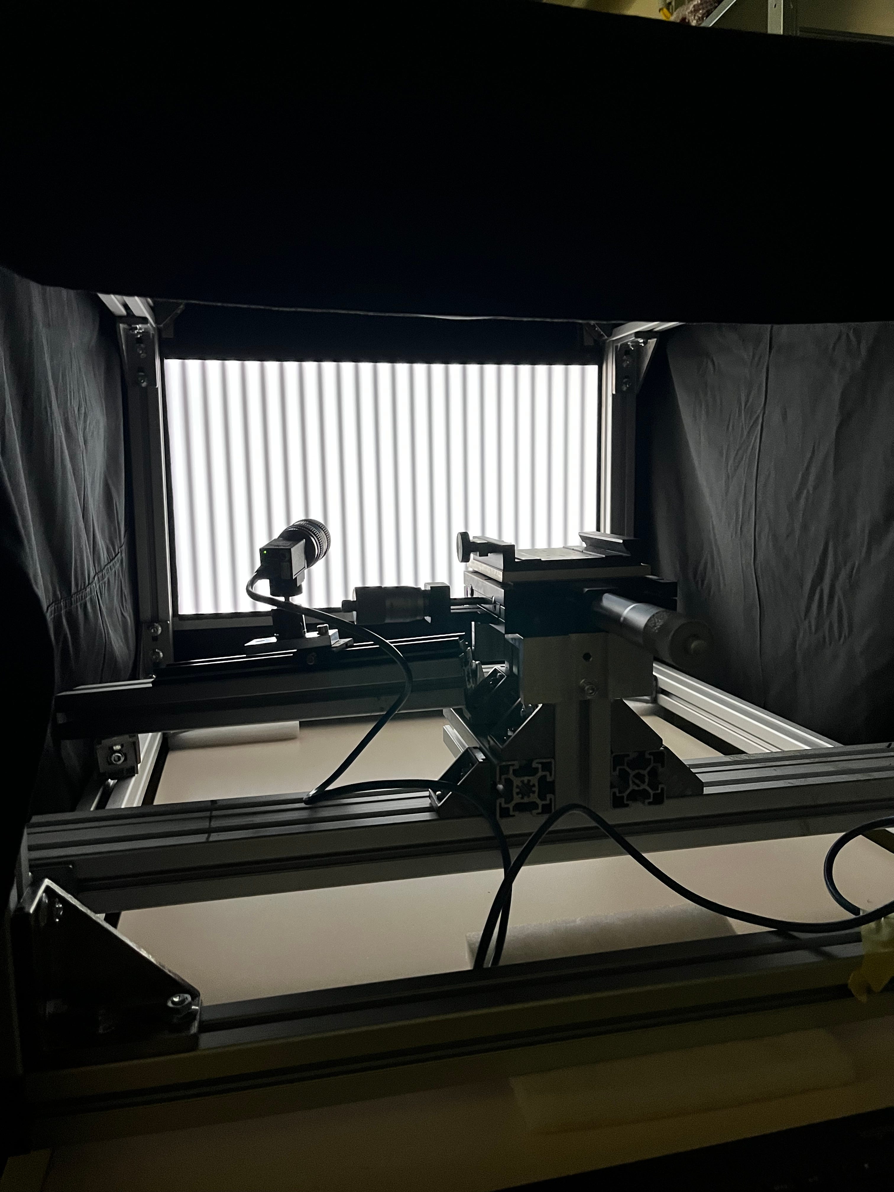
Fig. 2(b) shows the setup during the data acquisition. The camera in this photo is mounted on the rail (axis 3). Thick light-absorbing fabric protects the setup against stray illumination.
2.1 Experimental parameters and procedures
For consistency, the parameters of the lens (focus, aperture) were fixed in the beginning of a study. The focus was set at around the screen’s position, when observed from the micrometric platform; minor residual un-sharpness protected the data from undesirable moiré effects.
Before the actual data collection, we drove all electronic components at full speed/intensity for more than one hour so that they could reach constant temperatures. Even in the absense of air conditioning, we believe that the ambient air temperature remained stable to at least 1° during our recording session (about 2 hours) due to the large volume of the experimental hall.
Using our setup, we have collected data from 34 camera positions. At each position, the camera remained static, while the screen looped through a sequence of coded patterns. A custom Python program displayed each 4K pattern in fullscreen mode, waited 0.3 s for the intensity of LCD pixels to settle, and then initiated the recording. Each pattern was captured 10 times with
the exposure of 15 µs, and these frames were averaged before saving in 16-bit PNG format in order to reduce the noise. Due to fast gigabit Ethernet connection to the camera, this procedure did not cause any noticeable delays.
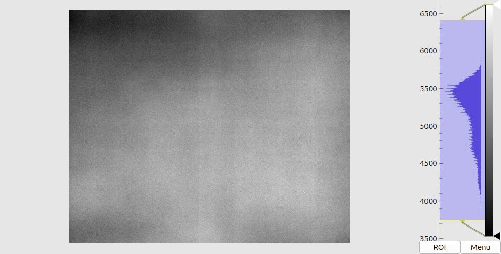
A sample recorded image is shown in Fig. 3(a). We observe sufficient (70-90%) utilization of the dynamical range of the camera and the absense of under-/over-saturated pixels.
2.2 Collected datasets
Of the 34 calibration datasets, the first six were intended to test the reproducibility of data and the stability of the resulting extrinsic parameters. The camera was mounted on the 2-axis platform with its knobs set to x = 0, z = 0. The data collection then proceeded as follows:
The dataset 0 was recorded at the basic position x = 0, z = 0;
The dataset 1 followed immediately after that, with no movement in between; • Before shooting the dataset 2, we have made a “roundtrip” with the x-knob: turned it to 1 mm (one full rotation) and then back to 0;
The dataset 3 was taken after a similar “roundtrip” of the z-knob to 1 mm and back;
The dataset 4 was taken after a “roundtrip” of the x-knob to 10 mm and back;
Finally, the dataset 5 was taken after a “roundtrip” of the z-knob by 10 mm.
The poses 0-5, therefore, have been technically collected at the same (basic) camera position.The deviations between the outcomes (decoded data and calibrated positions) for these poses then may characterize the decoding stability and/or the mechanical precision of the mounts.
Continuing where the previous series has ended, the subsequent five datasets were recorded as the camera was shifted to x = 5 mm, 10 mm, ..., and 25 mm (the z-knob remaining at 0). In other words, the projection centers for the poses 5-10 should be ideally separated from each other by a distance of 5 mm and belong to a common straight line in 3D.
Similarly, for the datasets 11-21 we have first returned the camera to the basic pose and then recorded data at z = 0, 5 mm, ..., and 50 mm with the x-knob fixed at 0. The logic here is the same as before, but with a longer range and a different direction of movement.
Further, the datasets 22-27 were shot with the camera mounted onto the “dovetail” rail. Since it has no micrometric screws, the positions of the slider could only be controlled visually based on printed 1 mm-ticks. Denoting the respective coordinate as l, we have moved the camera to l = 0, 50 mm, ..., and 250 mm. While these values may in reality be off by about 1 - 2 mm, the respective poses should still align in 3D with a good accuracy.
During the recording of the final series of poses (28-33), the camera was each time freely positioned in front of the screen. When choosing the perspectives, we attempted to ensure a sufficient range of observation angles and distances to the screen in order to better constrain the calibration, and at the same time maintain a reasonable frame coverage and image sharpness.
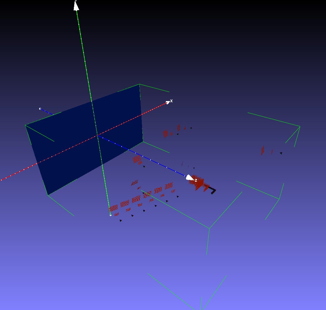
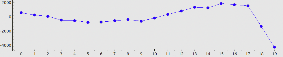
The resulting camera poses are visualized in Fig. 3. The screen is shown as a blue rectangle, the projection centers and orientations of the camera at each pose are indicated with small simplex-like placeholders, and the fans of view rays are shown as pairs of red grids.
3 Coding patterns
The pattern presentation pipeline works as follows. First, our custom encoder generates “raw” patterns as grayscale arrays with the native screen’s resolution and pixel values between 0 and 1. We then linearly re-scale the values to the range [0.1, 0.95] in order to avoid strong non-linearities near the endpoints on the screen’s intensity curve. After that, we raise the values to the power γ′ = 1.0/2.25 = 0.4444 in order to “undo” the default gamma-correction, which is typically
applied by the display and/or the operating system; in our case, its “strength” was found to be γ ≈ 2.25. Finally, we save the patterns as 16-bit PNG files and display them using low-level graphics functions, avoiding any further pixel value transformations.
Apart from the global gamma-correction, most MAT algorithms assume a linear transfer function between the grayscale values in the “raw” patterns and those recorded by the camera. In general case, however, some degree of non-linearity may remain (due to, e.g., the pixel technologies of the screen or the camera, or non-ideal electronics). When left un-corrected, it may increase random errors and/or introduce biases into the decoded spatial positions.
If our goal accuracy was at the level of 0.1 mm or worse, we could safely neglect such effects and devise a compact pattern sequence, robust even in the presence of strong pixel noise. Here, however, we aim to achieve data, consistent to about 10 µm. To that end, we have designed a sequence of 58 patterns that corrects residual non-linearities of transfer functions in each pixel, ensures the best practical decoding uncertainty in most (maybe not all) pixels, and facilitates a fair comparison between MAT-based and pattern recognition-based calibration. In the following sections we describe the roles of different patterns and the respective design parameters.
3.1 Calibration of gamma-curves
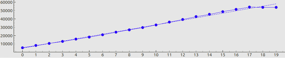
Our first 20 patterns belong to what we call a “gamma-sequence”. Each pattern is uniformly filled with some grayscale value; these values gradually increase in order to cover the range from the darkest (pattern 0, “raw” value 0.0) to the brightest (pattern 19, “raw” value 1.0) points.
When these patterns are displayed, the camera records images such as in Fig. 4(a). The nontrivial distribution of brightness in the frame is due to the non-uniform emittance of the screen, its angle-dependent characteristics, lens- and color-shading effects (vignetting), etc. However, in the context of spatial coding we are more concerned with the relations between the encoded and the recorded pixel values. Fig. 4(b) shows the evolution of recorded values in a fixed camera pixel over the gamma-sequence steps. We can see that the pixel value grows almost linearly, and only for the brightest patterns the curve “flats out”. If we fit a linear function to these points, the residuals will appear as in Fig. 4(c). The RMS fit error in this case will be about 1000 grayscale steps; compared to the total range of values, this amounts to a 1.5-2.5% relative error.
Note that the recorded values do not reach the absolute upper limit (65535). This means, that the “capping” in Fig. 4(b) is due to the screen not being able to display pixels at the full intensity (which may happen, e.g., due to matrix degradation). A proper solution here would be to re-scale the raw patterns more aggressively before the presentation (e.g., to the range [0.1, 0.9] or even further) and adjust the exposure accordingly. Unfortunately, we have noticed this problem only after the data collection had ended, and were not able to repeat the experiments. In what follows, we describe an alternative technique, which can partially compensate for sub-optimal data quality and significantly stabilize the decoding in other challenging situations.
The key observation here is that the “capped” behaviour of the curve in Fig. 4(b) is a stable systematic effect: by inspecting multiple pixels, we see that stochastic deviations on top of this general shape are relatively small. This means, that we can fit some smooth non-linear curve to these points, and it will capture the true local transfer function with small fit errors.
Our gamma-sequence decoder does just that. For each pixel, it fits a non-linear function to the 20 recorded values such as in Fig. 4(b). By inverting that function, it creates the respective “linearization” mapping. All the subsequent recorded values (which encode the spatial position on the screen) are “corrected” by this mapping before being passed to the respective decoder.
This pre-processing restores the linearity assumption, critical to these advanced codes. For our data at hand, the gamma-sequence-based correction has reduced the residual relative RMS errors (non-linearities and stochastic noise combined) down to the level below 0.5%, which is sufficient for high-quality decoding. Note, however, that the procedure is universal and may apply to other types of non-linear behaviour of screens and cameras.
3.2 Spatial coding sequence and synthetic tests
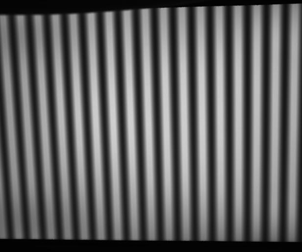
Our next coding block uses 18 + 18 patterns to encode x- and y-coordinates on the screen, respectively, using the well-known cosine phase-shifted patterns [6]. For both directions, we postulate the same three wavelengths and phase shift counts in order to ensure isotropic decoding uncertainties. The period of the finest fringes is about 2.6 mm on the screen, or about 14.2 screen pixels. This is sufficient to avoid non-linear effects, which may appear due to the interference of patterns with the underlying pixel grid.
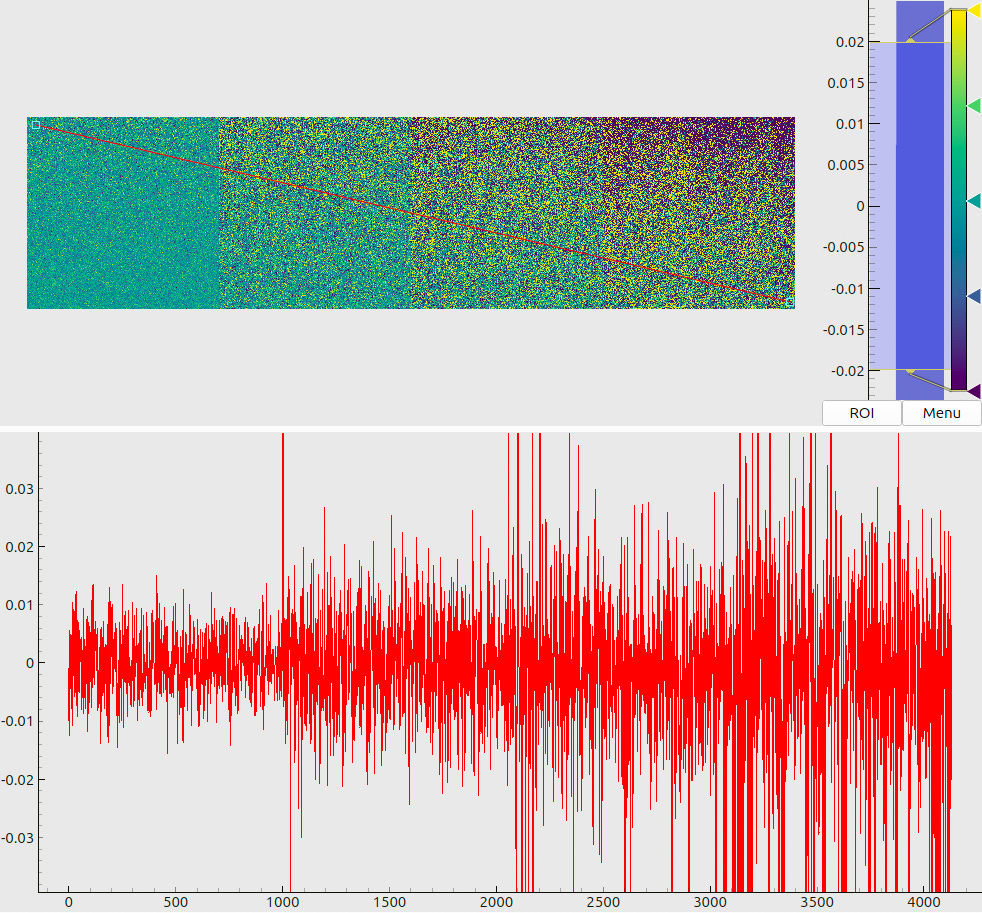
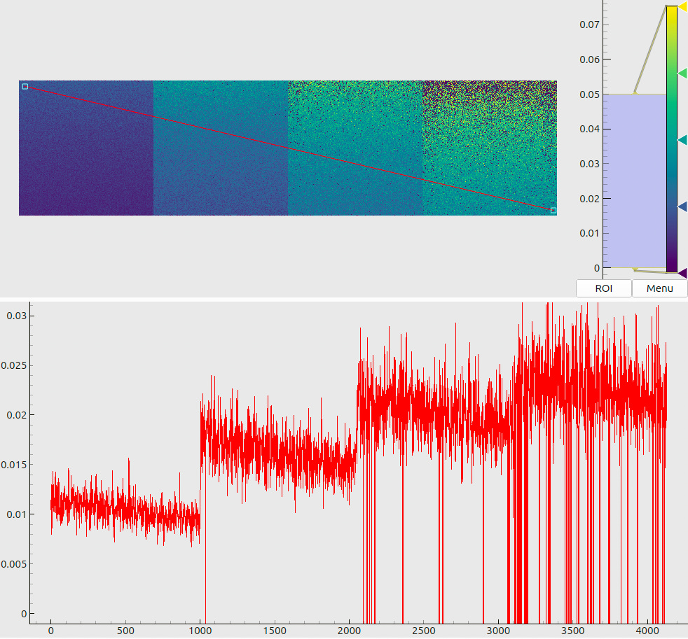
The expected performance of the code has been evaluated with the following procedure. First, we have encoded some valid screen coordinates in a window of 4096 x 1024 pixels. After that, we have applied a linear re-scaling to these patterns, and then added random Gaussian noise to each pixel. The parameters of these manipulations were specific to each pixel and were modulated by the maps in Fig. 5(a) and (b)1.
After the application of transforms, we obtain images such as in Fig. 5(c). These may be interpreted as “synthetic camera frames”, where each pixel has been captured under certain conditions. First, the decoding contrast linearly changes between 0.5 on the top side of the image and 1.0 at the bottom (the stripes in Fig. 5(c) appear “fainter” at the top). Second, each image
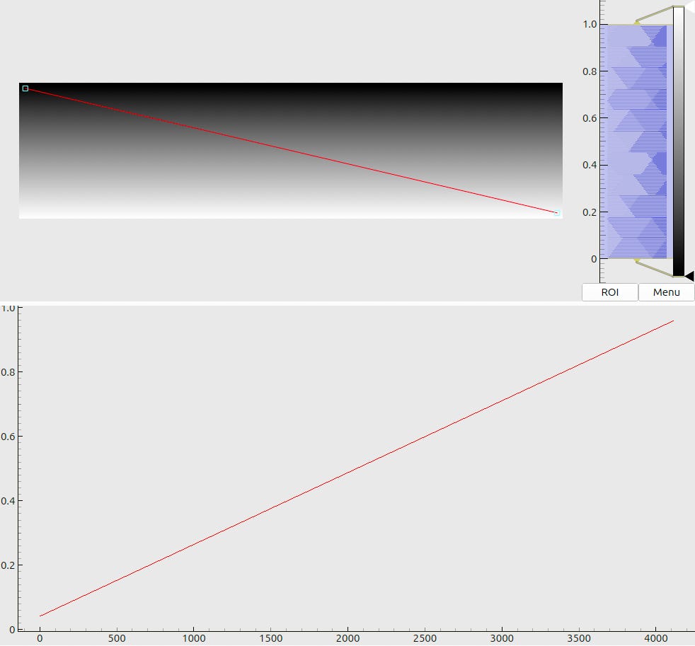
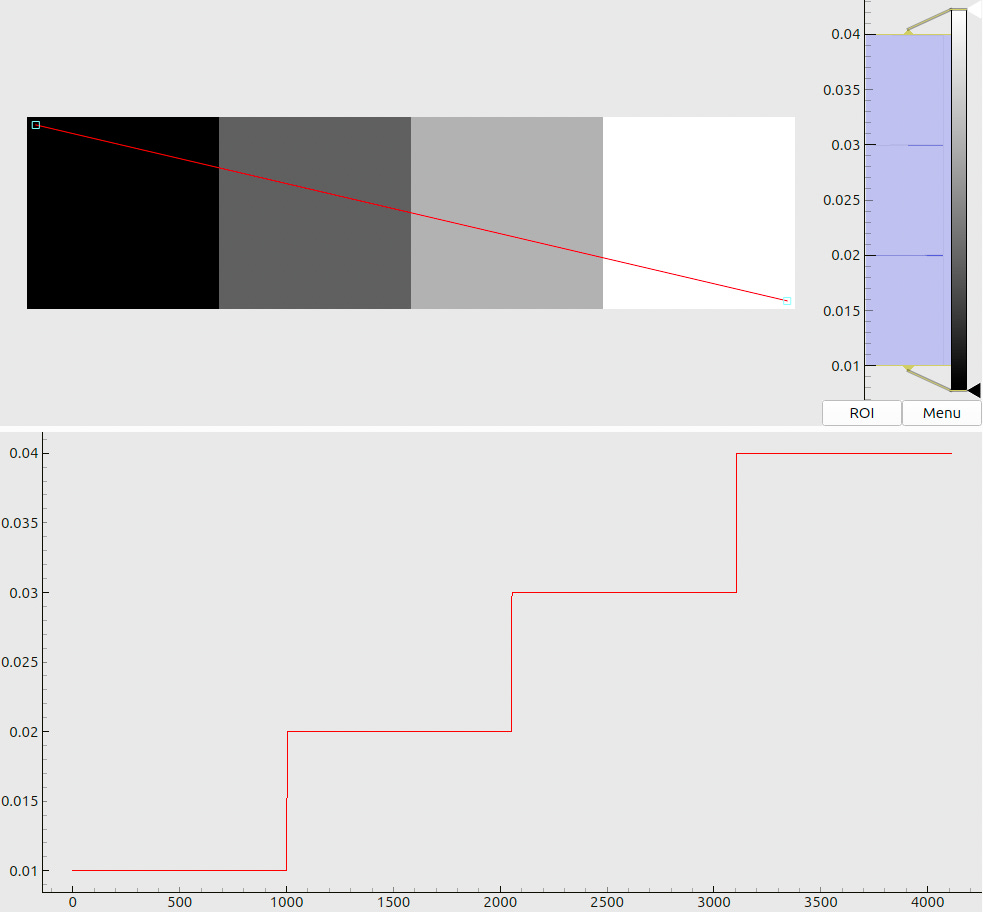
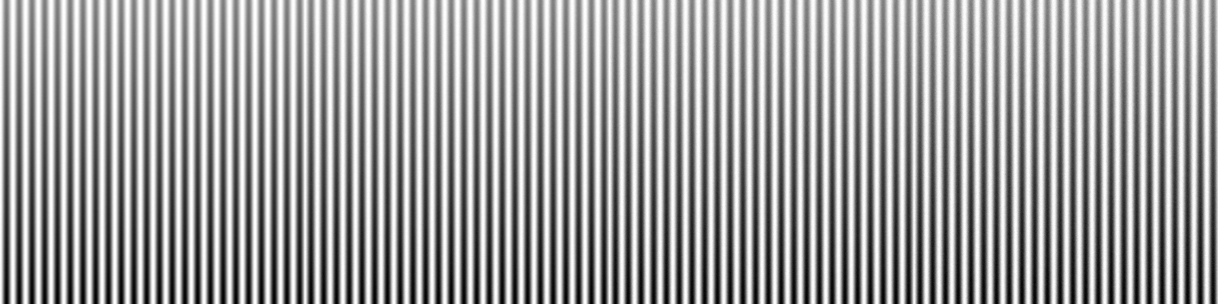
is split into four parts of 1024 x 1024 pixels. In these panels, the levels of added noise are 1%, 2%, 3%, and 4%, respectively (the rightmost part of the image appears “fuzzier”).
The modulated images are then passed to the decoder, which recovers the screen coordinates and estimates the respective uncertainties. Since the ground truth coordinates are known, we may then derive the actual decoding errors (Fig. 6(a)) and compare them to the predictions
(Fig. 6(b)). The analysis of these plots allows us to make the following statements:
For the decoding contrast above 0.5 and relative noise below 1% (as expected from the gamma-curve calibration, Sec 3.1), we may expect decoding errors of about 10 µm;
The predicted uncertainties agree with (or slightly over-estimate) the actual errors;
The decoding remains relatively stable (few failures, consistent errors) even for the noise levels of 2-3% as long as the modulation contrast exceeds approximately 0.7.
3.3 Verification chart and CharUCO board
So far, we have explained the roles of the first 56 patterns. The last two displayed patterns are not needed for the MAT per se, but are reserved for tests and comparisons.
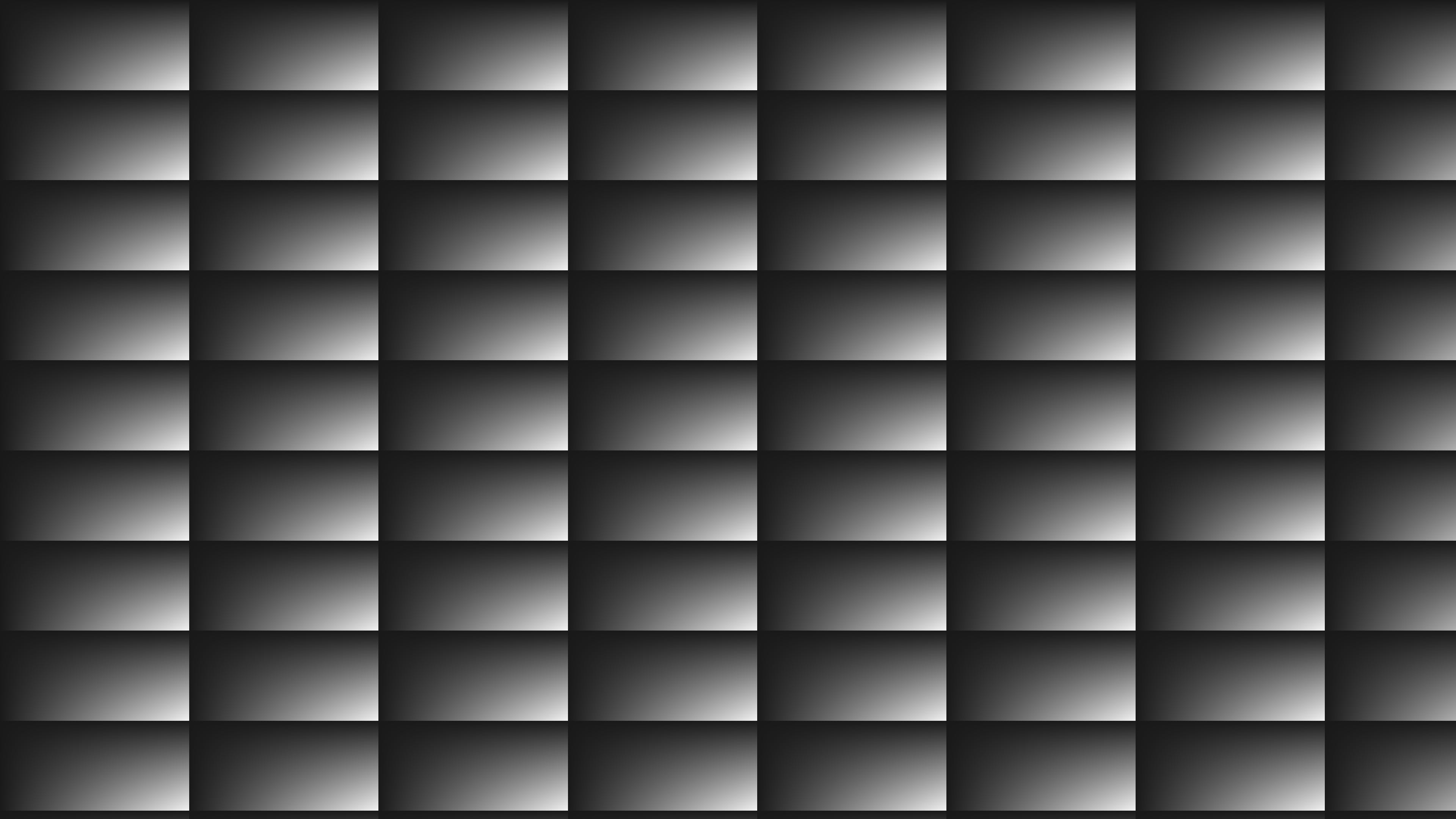
One of them is a verification chart (Fig. 7(a)), which is intentionally made asymmetric and contains rectangular blocks, filled with black-to-white gradient. By inspecting the respective camera images, a human operator can check the orientations of all axes and validate the capture quality.
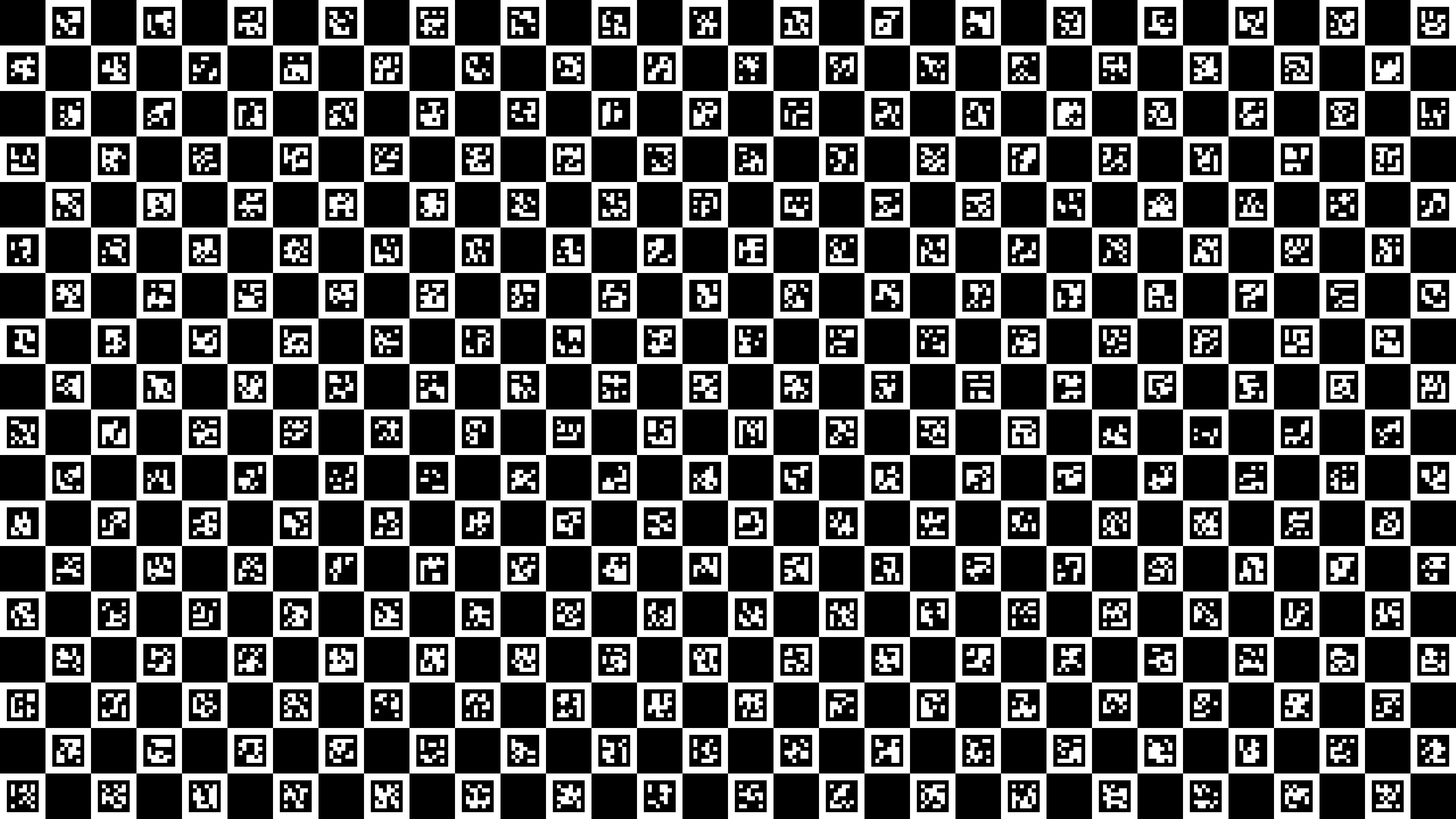
The second additional pattern is a 32 x 18 CharUCO board (Fig. 7(b)). Its geometry is known; it is photographed exactly as the other patterns and from the same camera poses. In Sec. 5, we use the respective images in order to perform a standard OpenCV detection and camera calibration, and compare the outcomes to MAT-based results.
4 Processing of calibration data
During the data acquisition, we have collected 58 5-megapixel images for each of the 34 camera poses. Their decoding is a relatively demanding calculation, but it can be efficiently parallelized. Our custom code, running on an RTX 4070 videocard, spends about 2-3 s per dataset. The resulting 34 multi-layer arrays contain the following values for each camera pixel:
x, y: coordinates of a point on the screen in mm;
△x, △y: estimated decoding uncertainties in mm;
q: decoding status (success of failure);
A: relative modulation contrast of the code (0 to 1);
△g: estimated relative grayscale noise level (0 to 1);
... a few additional parameters, describing local non-linear transfer functions (Sec. 3.1).
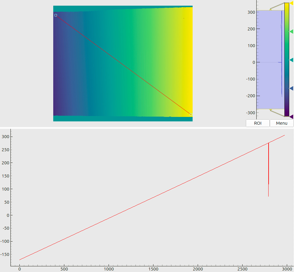
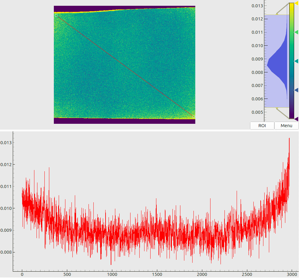
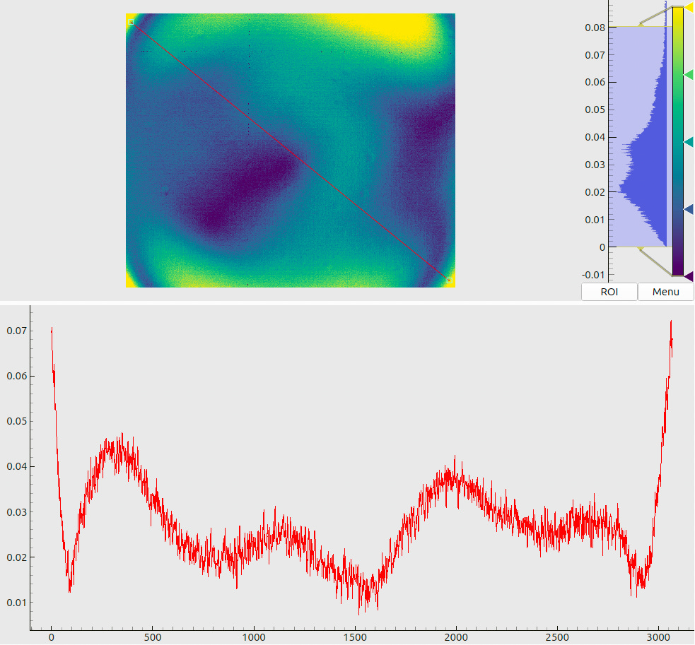
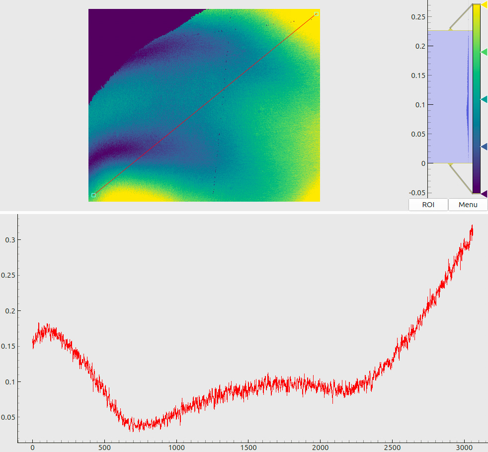
Two sample maps (produced for the same pose as Fig. 3) are shown in Fig. 8. The panel (a) shows the decoded x-coordinates, where we see a smooth gradient, indicating rather stable decoding without excessive “outbreaks” or failures. The panel (b) tells another important message: we observe that most of the decoding uncertainties end up slightly below 10 µm, which agrees with the design goals for our coding sequence (cf. Sec. 3.2).
4.1 Filtering of decoded datasets
When inspecting the plots in Fig. 8, we may notice some artifacts. First, there are isolated pixels where the decoding has failed (cf. a “dip” in the data profile in (a)). They could be expected based on the results of Sec. 3.2, as the local stochastic noise may randomly exceed the “stability limit” of 2-3%. In fact, by adjusting the decoding parameters we may reduce the number of such “outlier” pixels, but the typical decoding uncertainties (cf. the histogram in Fig. 8(b)) will slightly increase. The opposite is also true: we may extract more accurate coordinates from the same data, but the decoding in general will become less stable. Further, we may notice increased estimated errors at the screen boundaries. This can be explained by an interplay between the sharply bounded emitting area and the blurring kernels.
These and other optical effects may lead to minor biases in the decoded coordinates. Therefore, we exclude such “untrustworthy” spots by rejecting (declaring invalid) the pixels where
estimated uncertainties △x or △y exceed some threshold;
modulation contrast A falls below some threshold;
outbreaks in x or y exceed some level, relative to median values in the neighbourhood.
After these pixel-wise filters, we apply a binary erosion operation with a small radius (3 pixels) to all validity maps in order to remove any “suspicious” or “shaky” pixels on the boundaries.
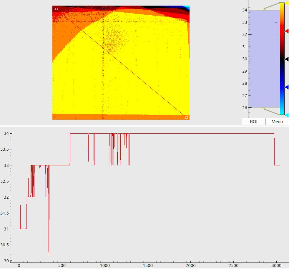
For the resulting “cleaned” datasets, Fig. 9 shows a global coverage map, i.e., the number of valid registrations for each camera pixel. The first thing we notice is the solid coverage, with at least 26 well-detected reference points in each pixel. Second, uneven contours in e.g. the upper-left corner of the map stem from the thresholded coding contrast: at some view angles, part of the screen appears too dim for stable decoding. Third, we see multiple isolated excluded defects, which collectively group into several “fuzzy lines” in the map. We have traced the origin of these artifacts to the secondary reflections of the aluminimum frame, illuminated by the screen, in the screen itself (cf. Fig. 2). Such effects are not a critical issue for our present experiments, but they should be taken into account in the design of any future high-accuracy machines.
4.2 Quality of decoded data
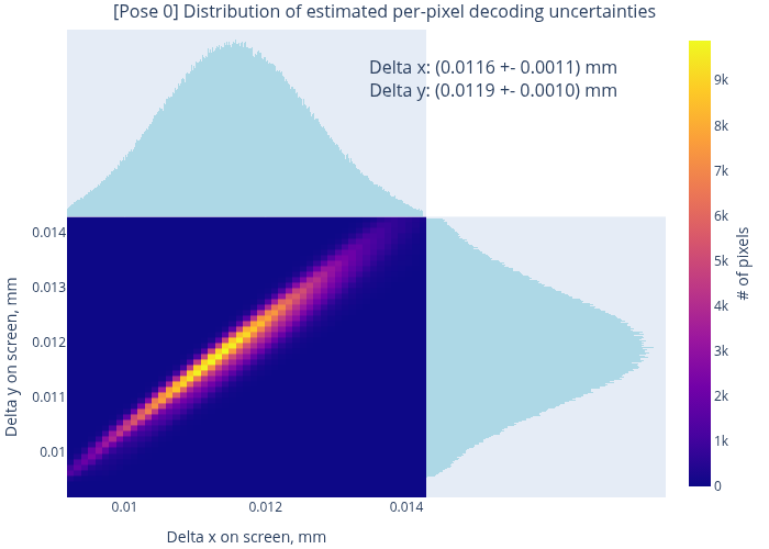
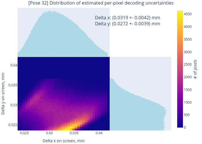
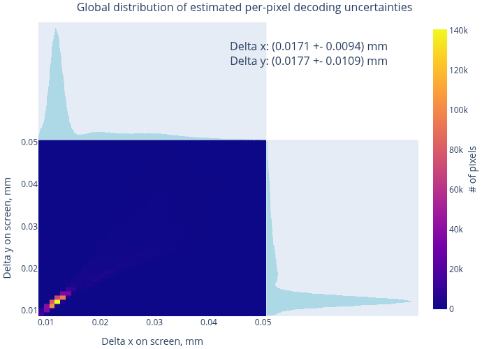
While such maps as in Fig. 8 are quite informative, they do not necessarily facilitate the reasoning about the global data quality. Fig. 10 presents a slightly more condensed representation of the same decoding results. First, we may compare the distributions of estimated decoding errors in some “good” (a) and “bad” (b) datasets. The typical errors in these cases end up around 11 µm and 30 µm, respectively. In the latter case, the screen has been significantly out of focus, and our data quality metrics reflect that. Nevertheless, we have enough “good” data, and the global errors (c) end up about 17 µm on average (cf. bi-modal structure of histograms).
4.3 CharUCO board detection
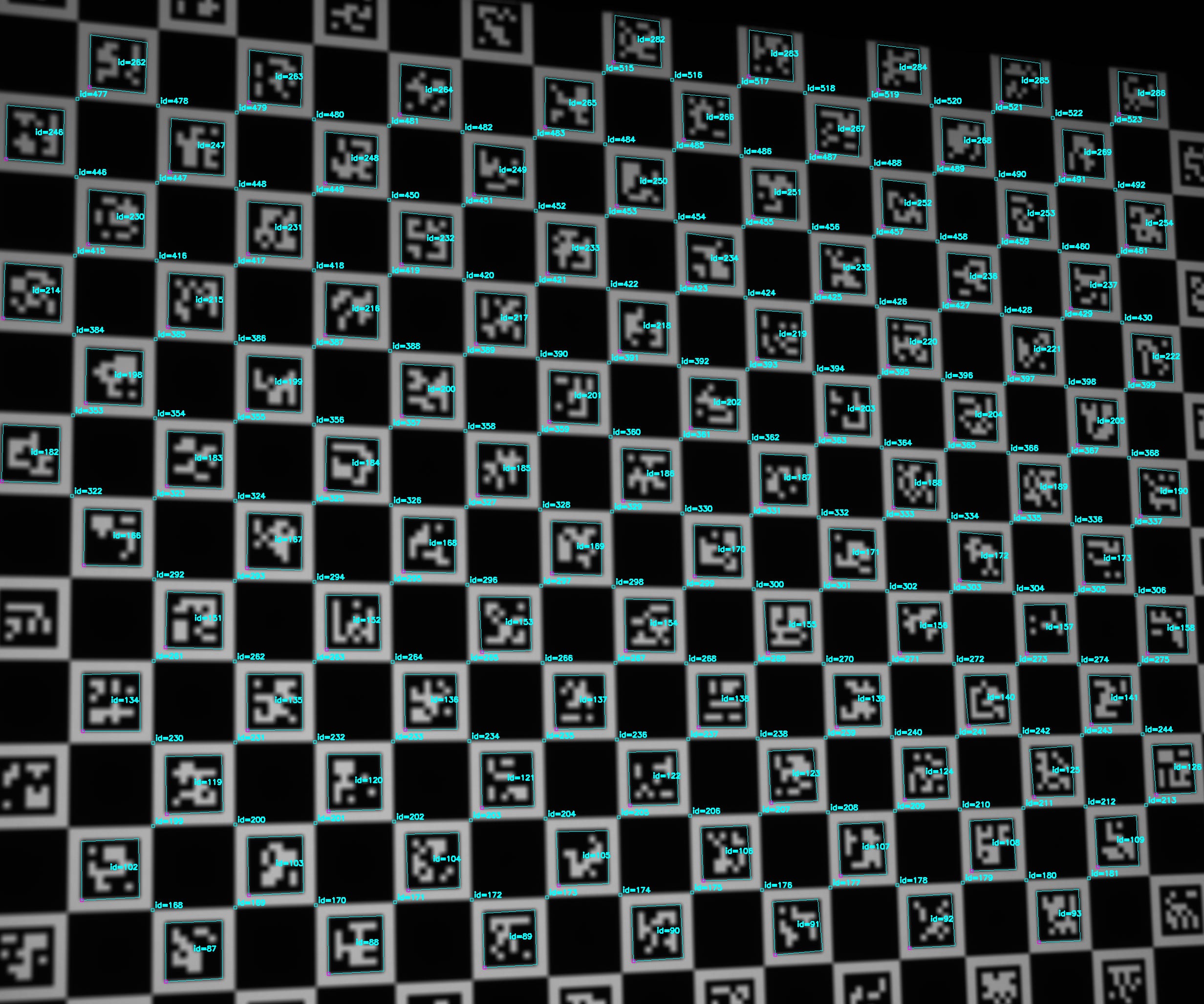
For CharUCO patterns, introduced in Sec. 3.3, we have built a separate detection pipeline using the OpenCV library [1, 3]. An ArUCO detector finds all valid markers in the image, and a checkerboard detector then finds the respective cell corners (Fig. 11(a)). It is these corners that we use for camera calibration, since the marker coordinates are in practice less stable.
The benefits of this technology appear obvious: we can collect data from a single exposure (i.e., there is no need to build stable frames and precision mounts), the method is (at the first glance) insensitive to environmental conditions, the processing is fast, and well-optimized libraries are available on all major computing platforms (no need for expensive GPUs).
In practice, however, as many industrial computer vision experts know, in any non-trivial case one still has to collect multiple exposures in well-controlled environments, and high-quality detection requires that one has to fine-tune dozens of mysterious parameters. In addition to these relatively straightforward issues, one also has to procure sufficiently stable and accurate targets. While flat screens are generally manufactured to µm-level tolerances and can be found virtually everywhere, a large industrial calibration target can easily be more expensive than a similar-size screen and cause problems of its own. (For instance, one may have to deal with import control regulations, imposed on high-precision devices.)
Here, however, we are more interested in fundamental differences, which may impact the quality of calibration. Fig. 11(b) shows all 6364 detected points across all 34 datasets. We immediately notice a region near the frame boundaries, where no points have been detected.
This is, in fact, a common feature of pattern recognition-based methods, which require a certain neighbourhood in an image in order to detect a landmark (such as a cell corner). There exist also other mechanisms that may further increase this bias in the distribution of calibration points: for instance, a wide-angle lens may distort off-center markers beyond recognition. As another example, when a regular (non-CharUCO) chessboard is used, it must be fully visible in the frame in order to be registered; “non-central” shots then are more likely to be rejected.
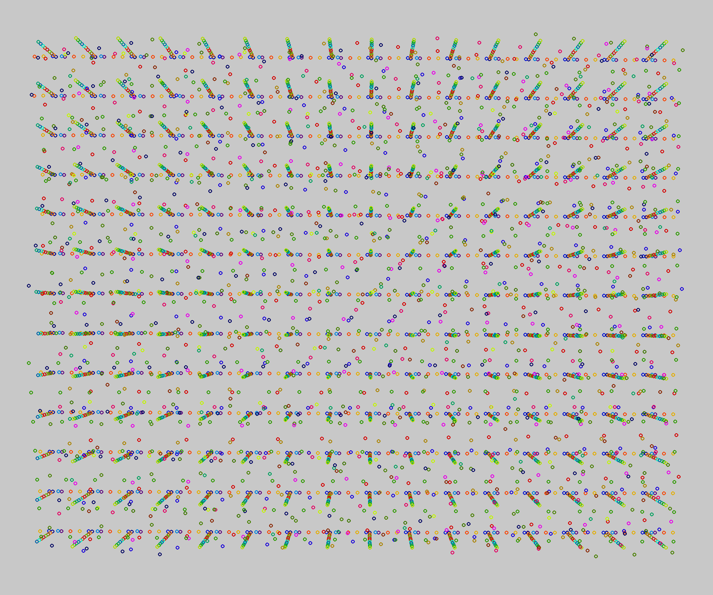
Apart from this effect, our 6364 collected reference points are remarkably stable due to very low pixel noise and high contrast, even despite some degree of un-sharpness. In fact, we believe that these results approach the limits of CharUCO algorithms for our recording conditions.
In order to get an idea about the quality of these points, we have compared the screen positions of the CharUCO reference points with the coordinates, decoded in our MAT data for the same camera pixels. The results, computed over all points and all poses, read as follows: the mean value and the standard deviation of the 2D displacements between the detected and the decoded screen positions are (30.0 ± 134.7) µm.
These numbers significantly vary for different datasets. For the “best” camera pose, we get (12 ± 87) µm, and for the “worst” (least sharp) images – (183 ± 548) µm. Compared to the
size of screen pixels (181 µm), we may technically claim agreement at the sub-pixel level. These numbers, however, are less impressive than those in Sec. 4.2. Nevertheless, as mentioned above, the results are perfectly suitable for high-quality calibration.
5 Calibration scenario I: CharUCO data and OpenCV model
Our first calibration attempt relies on the standard technologies (functions in the OpenCV library) in order to establish a baseline for comparisons with more advanced methods. Using the detected CharUCO points (Sec. 4.3), we calibrate the default perspective model. The adjustable intrinsic parameters of the model include the fundamental matrix (fx, fy, cx, cy) and six distortion coefficients (k1, k2, p1, p2, k3, k4) [1]. As we will see, this model is a good fit for our camera/lens combination, while remaining sufficiently simple and numerically stable.
The calibration completes in a few seconds and reaches the residual RMS RPE of 0.956 pixels. We believe that this is a decent result for a 5-megapixel camera. The calibrated camera positions are shown in Fig. 3(b) and also agree with our experimental design and intuition.
Unfortunately, the standard function does not provide us much additional information about the calibration quality. We may receive RMS RPE values for individual poses, but they are scalars
and tell us little about the localization of errors in the field of view, nor disclose their statistics. Also, RPEs do not directly characterize the model’s performance in 3D.
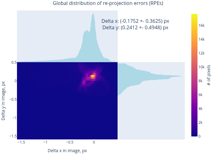
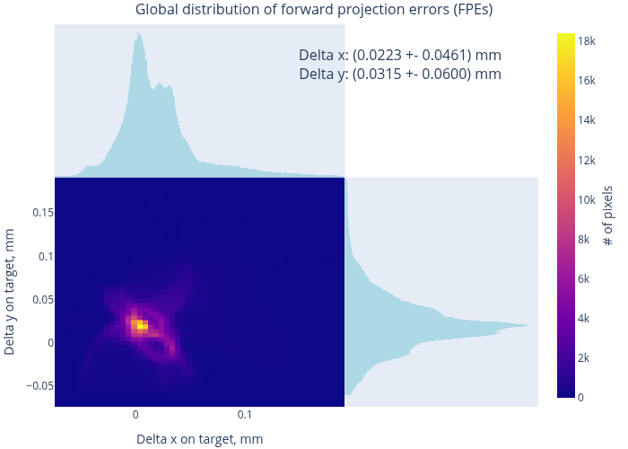
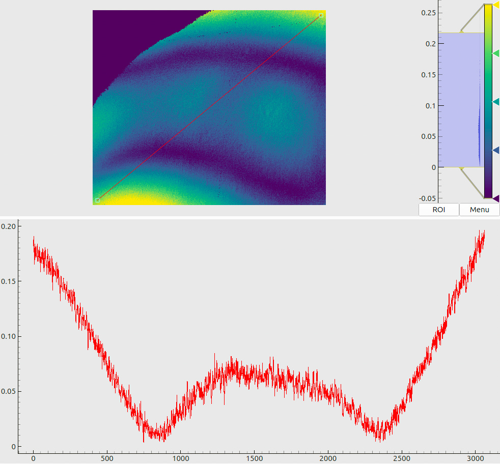
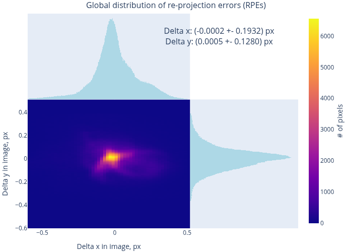
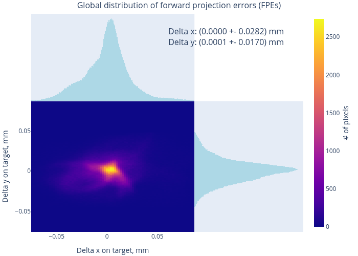
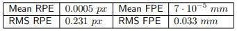
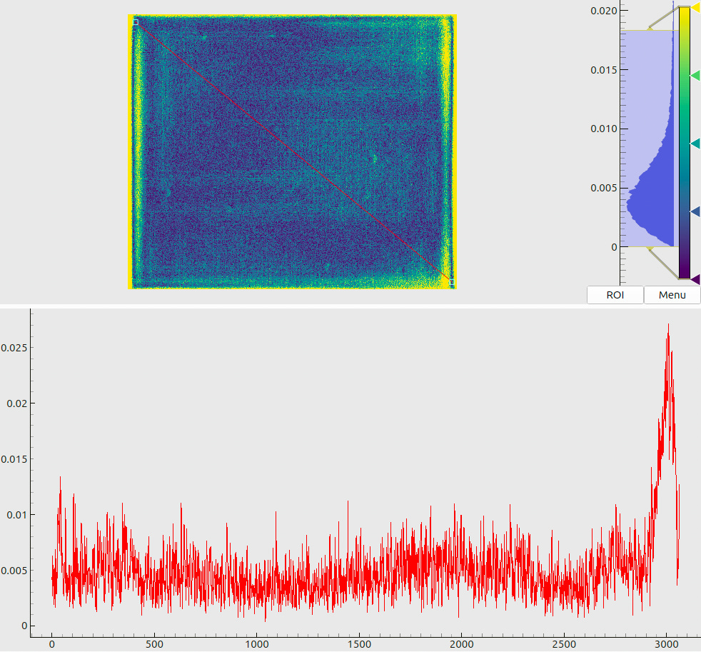
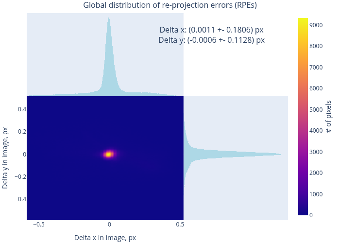
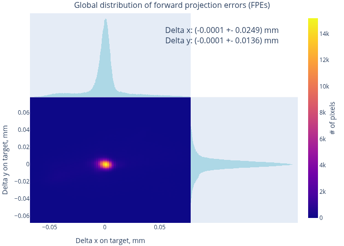
Therefore, we evaluate the quality of the resulting model using the MAT data. Fig. 12 shows the model-to-data consistency in terms of forward projection errors (FPEs) for two datasets – a “good” and a “bad” one. In the first case, the typical residual errors are at the level of 20 - 40 µm (cf. the embedded histogram), and in the second – at about 50 - 150 µm. A more general overview can be found in Fig. 13, which presents the distribution of RPEs and the FPEs, computed over all datasets. Condensing these results to global integral values, we find:
Here are a few conclusions that can we draw from these plots and numbers:
The maps in Fig. 12 are remarkably “flat”, especially in their central parts. Further, the peaks in Fig. 13 are well centered near zero. Therefore, we conclude that our MAT data are very well consistent with the model, calibrated on CharUCO points, and that there is no conflict between the two types of data within their respective statistical uncertainties.
The MAT-based RMS RPE is significantly lower than 0.956 pixels, reported by the OpenCV calibration. Therefore, the bulk of the latter value originates from the random noise in the detected reference points. Nevertheless, the model is “stiff” enough to not overfit to these variations, and has indeed captured the true imaging geometry of the camera.
Extending the logic of the previous point, we state that the reported RMS RPE inadequately characterizes the final calibration quality (which is better than that number implies).
Comparing our MAT-vs-CharUCO discrepancies in the data (Sec. 4.3) to the global RMS FPEs for the “good” and “bad” datasets, we see that the FPEs in the “bad” case end up lower than what could be expected. We believe that this fact illustrates a stronger degradation of CharUCO data quality as the image goes out of focus, compared to the behaviour of MAT data. The model could still be well calibrated for these poses, but it had to deal with a stronger noise than necessary.
Inspecting Fig. 12 and similar plots for other camera poses, we generally observe higher errors in the corners and on the “margins” of the frame. This behaviour is consistent with the lack of CharUCO data in these regions (cf. Sec. 4.3). Had we allowed higher-order distortion parameters, we would observe no improvement in the basic metrics, but “wilder” (unphysical and arbitrarily directed) oscillating errors in the corners.
The error maps do not feature any pronounced common structures in the center of the frame (“circles”, “waves”, etc.). Therefore, we see no reason to extend the selected model with further types of distortions, supported by the OpenCV algorithms.

Generally, in this example we see a high-quality calibration of a high-quality camera. Our lens has been designed and optimized to match the OpenCV camera model, and the pattern recognition has done a great job establishing unbiased reference points with very low noise. Notice, however, that we had to significantly rely on MAT data in order to arrive at these conclusions.
6 Calibration scenario II: MAT data and OpenCV model
In our second scenario, we again use OpenCV and calibrate the same model with 4 + 6 intrinsic parameters. However, instead of relying on CharUCO detections, we now sample reference points over a uniform 37 x 31 grid from the decoded MAT data arrays (to the maximum of 1147 points
per pose, which lets us complete calibration in less than 10 minutes). This way, we may only utilize less than 0.02% of the available decoded points, but OpenCV, unfortunately, does not yet support dense calibration data.
Note that CharUCO points are uniformly distributed on the screen, but may land arbitrarily on the camera’s sensor. With our scheme, however, we uniformly sample the entire frame. This should stabilize higher-order distortion coefficients and suppress “wild outbreaks” of errors.
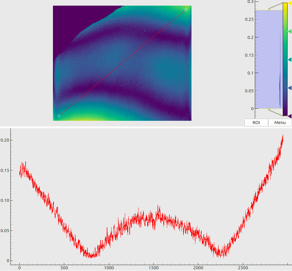
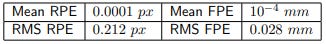
The Figs. 14 and 15 show the same metrics as the respective plots in Sec. 5. The global integral parameters (computed over all decoded pixels in all datasets) are as follows:
These values indeed significantly improve upon the baseline. The error distributions are concentrated around zero, and the corners of error maps appear much better-behaving. In Fig. 14(a), we even see some fine structures, which are probably associated with physical nonuniformities on the camera’s sensor or on the screen’s matrix. In any case, the residual errors now approach the scale of estimated decoding errors (Sec. 4.2), which set the limit on the achievable calibration quality. Large-scale structures, visible in maps such as Fig. 14, have relatively low amplitudes and cannot be immediately associated with any recognizable optical aberrations.
The methods of this Section are probably reaching the limits of the OpenCV model. For wellcompliant cameras and optics (such as what we have used here) they demonstrate O(10 µm)-level accuracy. Our MAT data ensure robust calibration and informative characterization of quality. Less “benign” devices – e.g., cameras with wider-angle lenses and complex distortions – could not be calibrated to the same standards. In the following Section we demonstrate a more universal approach, which takes the full advantage of MAT data.
7 Calibration scenario III: MAT data and free-form model
Our ultimate scenario uses the MAT data in order to calibrate a central free-form model, based on the concept of smooth generic camera calibration [6]. The model uses a 32 x 32 grid of cubic splines and optimizes its approximately 2400 intrinsic parameters via finite element method. The calibration algorithm does not minimize RPEs nor FPEs, but rather weighted 3D FPEs – a x^2-like metric, which naturally accounts for the estimated errors in each pixel (△x and △y).
This metric, discussed in details in the same reference, is optimal in the information-theoretical sense and is designed to consistently accommodate data of non-uniform quality.
The number of sampled points, needed to evaluate the discretized metric or the Jacobian, depends on the integration parameters and in our case reaches about 700000. We therefore may reasonably expect that the model “senses” all important features of the imaging geometry.
The calibration of such advanced models is only possible on a modern GPU with a sufficient amount of video RAM. Neglecting I/O operations, the calibration on an RTX 4070 video card took 10 minutes. This is not an inherent limitation of the algorithm, but rather a choice – as mentioned before, we can vary its computational costs in a wide range.
Again, Figs. 16 and 17 allow us to compare the outcomes to the previous results. The integral quality metrics (computed over all decoded pixels in all datasets) are as follows:
As we can see, the free-form model has slightly reduced the errors even compared to the scenario II. For “good” poses, our errors end up consistently at sub-10 µm-level, which is probably the best one can achieve for the present data. At the same time, the map in Fig. 16(b) appears
almost identical to that in Fig. 14(b). This fact illustrates the advantages of the weighted calibration metric: the points in “bad” datasets have larger decoding errors. Therefore, it makes no sense to reduce the respective FPEs/RPEs down to zero.
In order to better understand the changes in the model, responsible for these improvements, we have compared the view rays of the final model of Sec. 6 and the free-form model. This is not a trivial exercise; as discussed in Ref. [6], the freedom to choose the coordinate system of the camera may lead to artificially large discrepancies even between physically identical models. Therefore, we have first found an optimal 3D rotation between the two models, and then mapped the angles between the respective view rays. The resulting plot in Fig. 18 shows that the freeform model has “tweaked” the simple OpenCV model at the level of 10 - 50 µrad according to a very nuanced pattern. It is also worth mentioning that the calibrated camera poses in the scenario III differ from those in the scenario II only by a fraction of a micrometer.
8 Cross-checks of calibrated camera poses
The discussion of the calibration quality and the model accuracy has so far only involved the same data that we have used for calibration. However, one may argue that we are lacking independent confirmations. If, for example, the screen sizes in the documentation are wrong by a few percent, all of our decoded coordinates, camera positions, and all metric errors are also off, and we would not notice. In this Section, we present several consistency checks, facilitated by our experimental design and the nature of collected datasets (cf. Sec. 2.2).
8.1 Reproducibility of camera poses
The basic test of calibration quality uses the datasets 0-5, collected at the same position. We consider N = 6 respective calibrated camera positions (projection centers) p⃗ i (i = 0, ..., 5) as 3D points and compute some statistics:
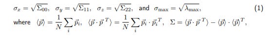
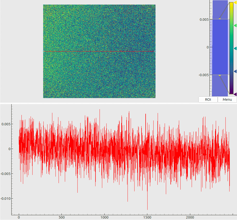
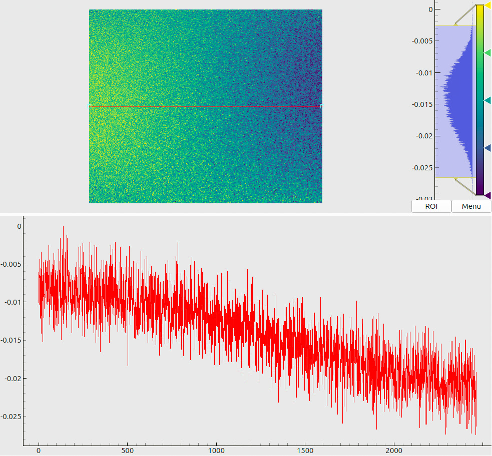
Figure 19: Differences between the decoded x-coordinates on the screen between (a) dataset 0 and dataset 1, (b) dataset 0 and dataset 5.
and λmax is the maximum eigenvalue of Σ. In other words, ϖx, ϖy, and ϖz measure the dispersion of calibrated camera positions along the respective axes, while ϖmax characterizes the maximum dimension of the six-point “cloud”.
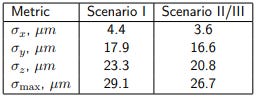
Table 1: Dispersion metrics for calibrated camera poses over the datasets 0, ..., 5.
Tab. 1 shows these values for all our calibration attempts (as mentioned above, the scenarios II and III have produced alsmost identical camera positions). We see that with better data we indeed obtain a slightly better consistency of poses along all dimensions.
The numbers, however, exceed our expected level of about 10 µm. We believe that this is happening due to the mechanical instability of the camera mount. Consider, for instance, pixel-wise differences between the decoded coordinates in the datasets 0 and 1, and a similar difference for the datasets 0 and 5 (Fig. 19). While the reproducibility of data without movement (a) remains safely within 5 µm (consistent with the expected decoding uncertainties), after several “roundtrip” movements within 10 mm the platform has accumulated a systematic shift in the data of order 15 µm (b). This may indicate a comparable residual displacement of the platform, accompanied by a small rotation (cf. the minor gradient in the map).
As an independent indicator of the calibration stability, we therefore also consider the distance between the calibrated camera poses 0 and 1, which is not sensitive to the quality of the platform. For the scenario I, this value is 6.9 µm, and for scenarios II and III, it is 2.8 µm. The improvement in the latter case originates clearly from the more accurate and abundant MAT data.
8.2 Linear motion along the x-axis
The datasets 5-10 correspond to shifts of the platform by 5 mm at each step along the x-axis. We analyze the respective N = 6 calibrated camera positions p⃗ i (i = 0, ..., 5) as follows:
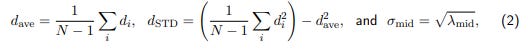
and λmid is the second-largest eigenvalue of the matrix Σ, computed for these poses (cf. Eq. 1).
The interpretation of these values is simple: d(ave) is the mean step length, d(STD) – the standard deviation of measured step lengths, and σmid characterizes the dispersion of points in the direction, orthogonal to the primary movement axis.
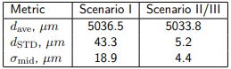
Table 2: Metrics of linear “steps” along the x-axis (datasets 5, ..., 10).
According to the values in Tab. 2, our advanced calibration scenarios indicate significantly more stable shifts and a more linear trajectory. The deviations of the measured step sizes from the expected value of 5 mm (5000 µm), however, requires a further investigation.
8.3 Linear motion along the z-axis
The same analysis as in the previous case can be applied to the steps along the z-axis (datasets 11-21); Tab. 3 summarizes the results. We again observe a very clear linear movement in scenarios II and III, and the step sizes are again larger than expected.
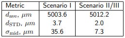
Table 3: Metrics of linear “steps” along the z-axis (datasets 11, ..., 21).
8.4 Linear motion at an oblique angle
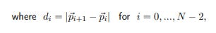
In our final linear test (datasets 22-27), we do not expect consistent step sizes. Therefore, we may only meaningfully compare the transverse deviations in Tab. 4. Again, the results in our scenarios II and III appear more consistent with the value of 55.7 µm. As in the first test(Sec. 8.1), a large part of this value should probably be attributed to the quality of the mechanical setup.
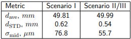
Table 4: Metrics of linear “steps” along the “dovetail” rail (datasets 22, ..., 27).
9 Summary
In this work, we have compared state-of-the-art and some recently proposed camera calibration methods in order to probe the practical limits of achievable calibration quality. Specifically, we have considered the method of active targets (MAT) for the data collection, and a multiparametric free-form model as the target representation for the intrinsic imaging geometry of a camera. Using a stable experimental setup with high-quality components, we have recorded MAT datasets as well as images of a static calibration target. The spatial code was designed to ensure 20 decoding errors of order 10 µm for some “normal” conditions; the posterior global estimated uncertainties for the collected data (target positions) ended up at the level of (17 ± 10) µm.
As reference data, we have captured CharUCO boards from exactly the same perspectives. According to our estimates, the noise in CharUCO points is at the level of 130 µm.
Using the CharUCO data and OpenCV calibration algorithm, we have performed the baseline calibration (scenario I). This has reached the RMS RPE value of 0.68 px and the RMS FPE of 85 µm. Overall, we believe this to be a very high-quality standard calibration.
In the scenario II, we have calibrated the same OpenCV model based on sub-sampled MAT data. This time, we have obtained the RMS RPE of 0.23 px and the RMS FPE of 33 µm. The calibration was significantly more stable and the error maps did not have any “outlier regions”.
Our final method (scenario III) has used the MAT data in order to calibrate a custom freeform model. While the integral metrics (RMS RPE of 0.21 px, RMS FPE of 28 µm) appear only slightly better than in the previous case, all error maps and histograms indicate an extremely stable and uniform model-to-data agreement.
In addition to these standard KPIs, our experimental design provides several cross-checks for the final extrinsic parameters. To that end, during the collection of some datasets we have mounted the camera on precision linear movement platforms. The standard calibration (scenario I) has demonstrated satisfactory results with 10↑40 µm deviations from the expected 3D metrics. In the scenarios II and III, the agreement of most control values was better, with typical errors reaching the level of 10 µm or less. However, as we have discovered during the analysis, the current tests were somewhat limited by the insufficient stability of the movement stages. Our conclusions from this study are as follows:
As suggested in [7], MAT data should be used whenever possible even for the standard models. With limited additional effort, they enable significantly more accurate calibration. Even more importantly, dense and rich data facilitate a significantly more detailed analysis of the calibration quality.
MAT in combination with free-form models can be an a solution for the most demanding applications. MAT-specific calibration metrics optimally extract information from the data, while the model is not limited by pre-defined simple types of lens distortions.
We believe that 10 µm sets the practical limit for the calibration of typical tabletop-scale machines, unless one uses exotic hardware and/or data from additional sensors. Many physical effects – un-sharpness, pixel structure, screen brightness, turbulence, temperature gradients, etc. – have to be accounted for in order to significantly reduce this value. That said, 10 µm would be a significant improvement for many industrial applications.
10 Open questions and further work
While the present work does illustrate some advantages of MAT-based calibration, it is certainly not the last word on the topic. In particular, the following questions require attention:
The experimental procedures must adopt the ML-inspired methodology [7], which avoid possible under- and over-fitting effects and produces extended quality metrics.
Once we reach the level of 10 µm in the model-to-data consistency, we should also consider the effects of non-ideal screen (e.g., refraction in cover glass and global deformations [10, 2]). According to our estimates, respective corrections to the decoded points in this experiment may be as high as 10 ↑ 50 µm in some pixels, which may e.g. partially explain the observed systematic deviations in the linear platform displacements (cf. Sec. 8.2, 8.3).
Similar studies should be completed with alternative lenses, which cannot be as well described by the standard OpenCV camera. A demonstration of calibration errors at the 10 µm level would be a powerful argument for the utility of free-form models. 21
Coding techniques may certainly be improved. In particular, it is possible to design shorter sequences with comparable properties. Alternatively, codes may be used to characterize the photometric sensitivity of a camera or its blurring properties (cf. Sec 3.1).
Acknowledgements
We are extremely grateful to Fraunohofer IOSB for providing us hardware and most of laboratory equipment in order to conduct these experiments, and personally to Dr. Jan Burke (SPR department) for many inspiring discussions and useful suggestions about the workflow.
References
[1] Camera calibration and 3d reconstruction. https://docs.opencv.org/4.5.2/d9/d0c/group__calib3d.html. [Online, accessed 20-June-2021].
[2] Jonas Bartsch, Michael Kalms, and Ralf B. Bergmann. Improving the calibration of phase measuring deflectometry by a polynomial representation of the display shape. Journal of the European Optical Society-Rapid Publications, 15(1):20, 2019.
[3] G. Bradski. The OpenCV library. Dr. Dobb’s Journal of Software Tools, 2000.
[4] A. K. Dunne, J. Mallon, and P. F. Whelan. Efficient generic calibration method for general cameras with single centre of projection. Computer Vision and Image Understanding, 114(2):220–233, 2010.
[5] L. Huang, Q. Zhang, and A. Asundi. Camera calibration with active phase target: improvement on feature detection and optimization. Optics Letters, 38(9):1446–1448, 2013.
[6] A. Pak. The concept of smooth generic camera calibration for optical metrology. tm – Technisches Messen, 83(1):25–35, 2015.
[7] Alexey Pak, Steffen Reichel, and Jan Burke. Machine-learning-inspired workflow for camera calibration. Sensors, 22(18), 2022.
[8] V. Popescu, J. Dauble, C. Mei, and E. Sacks. An efficient error-bounded general camera model. In Proc. 3DPVT, 2006.
[9] S. Ramalingam, P. Sturm, and S. K. Lodha. Towards complete generic camera calibration. In Proc. CVPR, 2005.
[10] T. Reh, W. Li, J. Burke, and Ralf Bergmann. Improving the generic camera calibration technique by an extended model of calibration display. Journal of the European Optical Society: Rapid Publications, 9, 10 2014.
[11] S. Reichel, J. Burke, A. Pak, and T. Rentschler. Camera calibration as machine learning problem using dense phase shifting pattern, checkerboards, and different cameras. In Bahram Jalali and Ken ichi Kitayama, editors, AI and Optical Data Sciences IV, volume 12438, page 124380P. International Society for Optics and Photonics, SPIE, 2023.
[12] C. Schmalz, F. Forster, and E. Angelopoulou. Camera calibration: active versus passive targets. Optical Engineering, 50(11):113601, 2011.
[13] T. Schöps, V. Larsson, M. Pollefeys, and T. Sattler. Why having 10,000 parameters in your camera model is better than twelve. In Proc. 2020 IEEE/CVF Conference on Computer Vision and Pattern Recognition, pages 2535–2544, 2020.
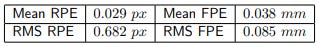
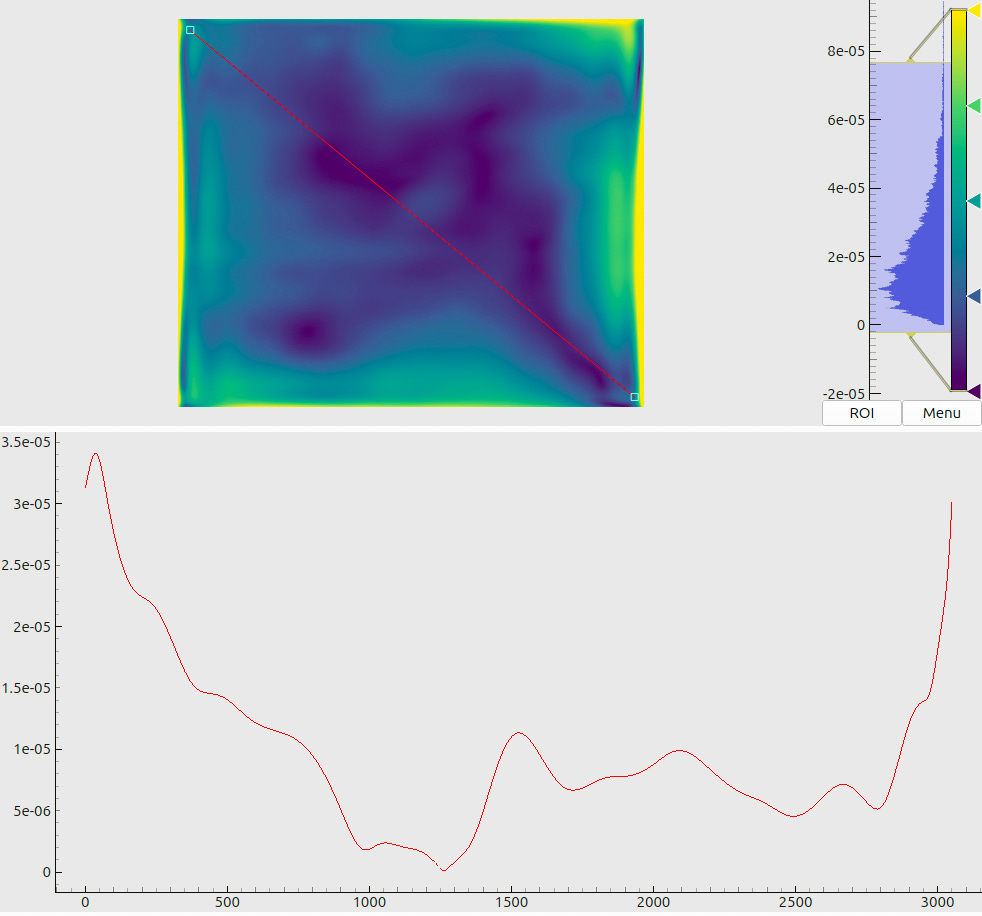
The meaning of combined plots such as in Fig. 5(a) and (b) deserves a short explanation, since the same layout is used many times throughout this document. The upper half shows a 2D color (or, in this case – a grayscale) map. The respective legend (a colorbar) is shown to the right of the map along with the global histogram of values. A red line, drawn on top of the 2D map, denotes a “region of interest” – a slice through the data array. The lower half of the plot then visualizes the profile of values, sampled along this line.